Understanding gradient descent

I totally expected to get started with coding at this point. After all, I have a great (basic) understanding of what a perceptron is, and how several of these are arranged in layers within a neural network. And it's intuitive to think of the network as a computer program (because it IS one, or at least in principle it could be). But turns out, the major focus of the "Machine Learning" is the "Learning" bit, so that's what we're going to be tackling now. (This post follows the previous article in this series so it's written as a continuation)

WTF is a cost function anyway?

So turns out, there needs to be some sort of a metric to tell the neural network, "Hey, what you're outputting is wrong!" and more importantly, for a way to tell it, "The output is wrong by THIS much". This is where the cost function comes into play. It's an elegant way to provide the cost of the network, so the higher this cost, the lower the accuracy of training. Our goal would be to minimize this cost to bring it down to close to zero.

The cost function is provided like so:

$$C(w, b) = \frac{1}{2n} \sum_{x} \| y(x) - a \|^2$$

where, w denotes all the weights of the network (in a weight matrix) and b represents the biases in a bias matrix, n is the total number of training inputs, y(x) being the desired output needed for a set of inputs to the network and a being the generated output of the network. We essentially calculate the MSE (mean squared error) of the network by getting the "diff" and then squaring this diff and then averaging the result out over all the training data. This is also called the quadratic cost. The $\frac{1}{n}$ is present to average out the result over n number of inputs, and the 2 is present alongwith the n so that it's easier when this value is differentiated and the square gets cancelled with this 2. It's just a random number to make life easier.

So we have the cost function. What now? Well, we need to optimize the cost of a multi-variate system, but to simplify things, let's consider a system with 2 variables/dimensions.

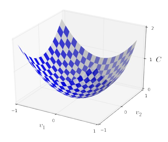
As you can see in this image, there is a graph of the cost function plotted between two variables v1 and v2. When we say we want to find the MINIMUM of this graph, it would mean the local minima here, which would be the bottommost point of the valley in this curve. And we can get there using a partial derivative of the cost method wrt each variable (v1 and v2 in our case).

$$\Delta C = \frac{\partial C}{\partial v_1} \, \Delta v_1 + \frac{\partial C}{\partial v_2} \, \Delta v_2$$

We want to be picking a value of $\Delta v$ such that $\Delta C$ is negative. This is because the gradient $\Delta C$ gives us the slope of the method and we want it to DECREASE down towards the valley we mentioned and not go up. We want to represent this nicely, like so:

$$\Delta C = \nabla C \cdot \Delta v$$

And now, we re-write $\Delta v$ in terms of $\nabla C$ too, by introducing a new variable $\eta$ (which is the learning rate):

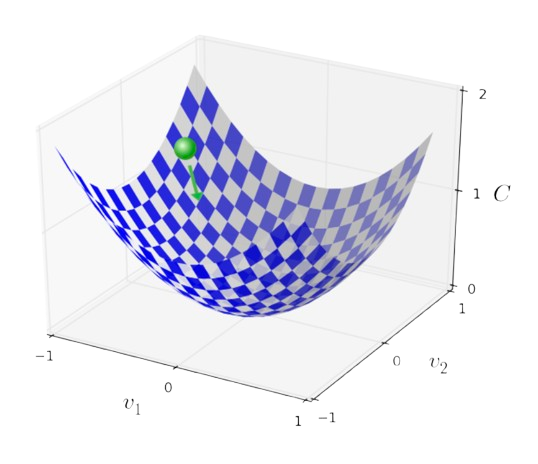
$$\Delta v = -\eta \nabla C $$

Here, the learning rate essentially tells us how fast or slow we want to be going down the valley. This is our first hyperparameter. This is something that we can adjust based on the network, and there isn't one solid answer to what the learning rate should be. There are advantages and disadvantages of it being too large or too small. Let's illustrate this using a ball that's tumbling down over the valley, but we get to control how far down it goes in a given step.

And THIS is how gradient descent works. The illustrations of the graph are overly simplified because the example here is only for two variables (over two axes), but in reality, we want to be dealing with millions of dimensions/variables. And a way we can represent n variables would be:

$$\Delta C = - \eta \left| \frac{\partial C}{\partial v_1} \Delta v_1 + \frac{\partial C}{\partial v_2} \Delta v_2 + \cdots + \frac{\partial C}{\partial v_n} \Delta v_n\right|^2 $$

Stochastic Gradient Descent

SGD (Stochastic Gradient Descent) is an optimized way of calculating gradients across many different inputs. This overcomes the issue of the performance overhead caused by attempting to calculate the gradient descent of a multi-variate network all at once. It does this by taking m amounts of inputs at a time in something called a mini-batch and then works out the gradient descent only for these inputs. And then this set of inputs is randomized so we arrive at the local minima faster per each step than attempting to get there in one shot.

We now have another hyper-parameter, which is m. These are going to come very handy when we want to be running some training/testing to build models optimized for higher accuracy. These are indicators of how well a model can perform, and are therefore some important variables that we can play around and set the best possible values that suit our use case.

SGD is kinda like the de-facto for figuring out the local minima of any multi-variate graph. So the process is simple:

• Weights and biases help the model make a prediction.
• Weights and biases need to be set in the right way for it to make an accurate prediction.
• Cost function tells us the total cost of the current network with current set of weights and biases.
• SGD is used to repeatedly modify weights and biases until it reaches a sweet spot where cost function is minimized.
• Hyper parameters like the learning rate or mini-batch size can be tweaked for achieving more accuracy and/or faster performance of the model during training.